Run sample script
After installation, you’re all set to launch your first simulation!
As a first exercise, open MATLAB and run the commands listed below from within the openstream folder, which will simulate an example of boiling two-phase flow in a uniformly heated tube followed by an adiabatic region. The OpenSTREAM mixture model will be used, which defaults to the Homogeneous Equilibrium Model (HEM) when the physical models are not modified by the user.
This is the quickest and easiest way to start exploring what OpenSTREAM can do, and to confirm everything is working smoothly under the hood.
% Clear existing variables from workspace
clearvars

% Import the necessary classes for inputs and solvers
import Inputs.*
import Solvers.*
import Solvers.Mixture.*

% Turn off warnings during input setup
warning off
% Create the input set using paths to model, options, geometry, and boundary condition files
inputSet = InputSet( ...
            modelFilePath         = './inputs/models.inp',  modelID    = 'TUTORIAL1', ...
            optionsFilePath       = './inputs/options.inp', optionsID  = 'DEFAULT', ...
            geometryFilePath      = './inputs/geom.inp',    geometryID = 'TUTORIAL1', ...
            bcFilePath            = './inputs/tutorial1.inp', ...
            sessionParentDir      = fullfile(pwd,'outputs'), ...
            overwriteSessionFiles = true, ...
            LOGMODE               = 'BOTH');

% Create a mixture solver object
mixSolver = MixtureSolver(inputSet);

% Solve
mixSolver.solve();

% Default axial plots
mixSolver.plotz();

% Save results
mixSolver.save();
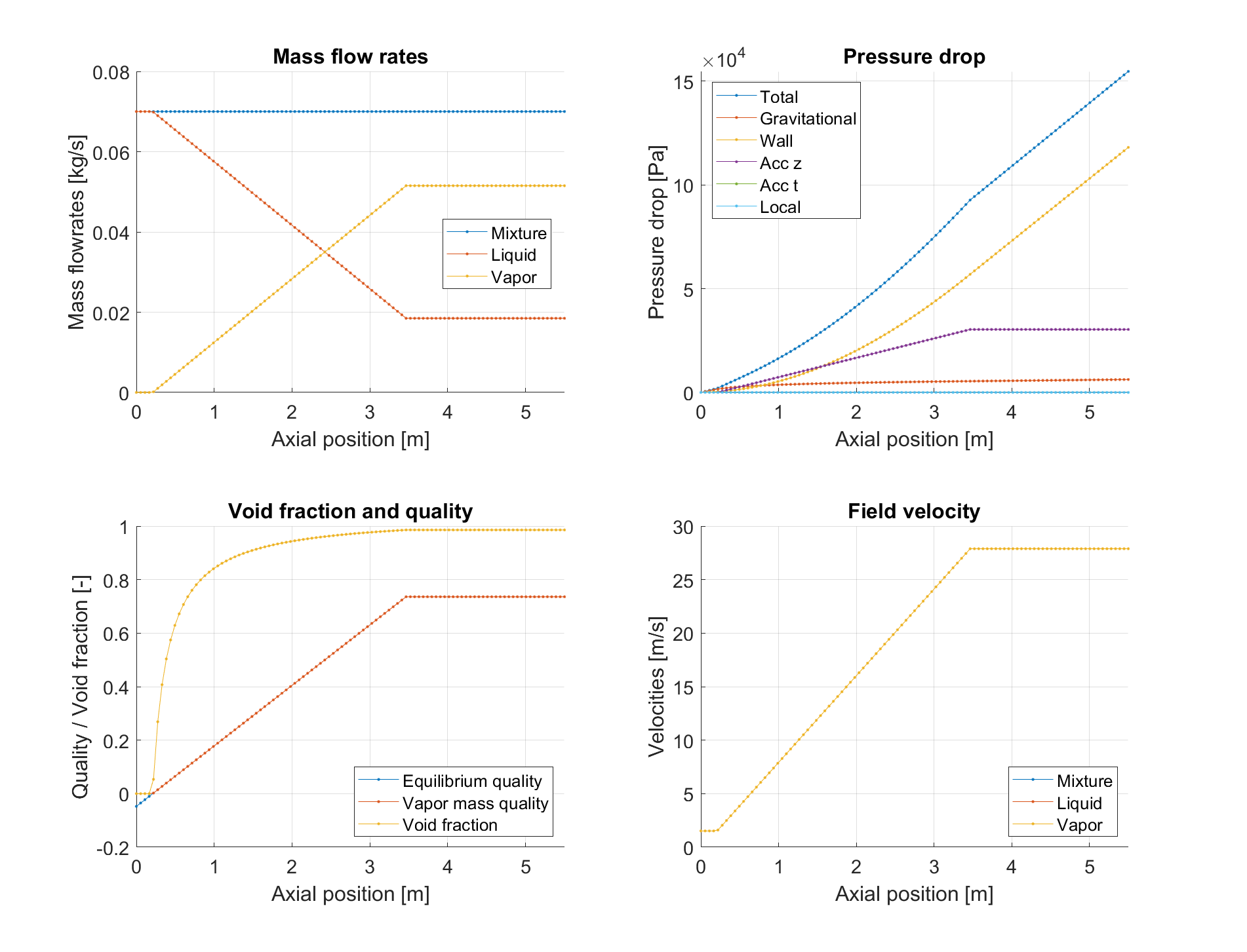
Sample figure of axial distributions of mixture parameters.